Portal User Guide and Manual

Land cover and its change analysis play an important role in providing crucial information for studying and monitoring ecosystems and their services for natural resource management. Assessment of land cover dynamics is essential for the sustainable management of natural resources, environmental protection, and food security. The land cover maps are primary data required for various other models including hydrology, ecosystem services, and weather forecast. National development plans use land cover as a basis for understanding changes in a country’s natural capital. The progress of governments’ efforts towards reducing emission cannot be measured without monitoring of land cover change. However, many developing regions lack the capacity to produce timely, accurate, and comparable land cover data products sufficient to meet their needs.

The Lower Mekong (LMR) and Hindu Kush-Himalaya (HKH) regions are both experiencing an acceleration in the rate of land cover change that is impacting the long-term sustainability of ecosystem services including food, water, and energy. Local decision makers are using infrequently updated national maps with no ability to monitor in a timely or integrated fashion. Furthermore, existing classification systems do not always meet the users’ needs, data products are often not widely shared between agencies and institutions, and accuracy assessment is often lacking. The users and developers of these maps are typically from different organizations with different priorities and technical understandings. These differences pose a variety of challenges that often create roadblocks to the effective use of appropriate land cover data for policy formulation, planning, management, and other decision contexts. As a result, global land cover products are frequently used as the best available alternative when appropriate and timely maps are not available at the regional, national, or sub-national levels. The global products have their limitations in that they have been created using different sensors and different techniques and vary in spatial resolution and classification typology, and contain inconsistencies on global scales. These inconsistencies hinder more widespread and effective use of land cover data to valuably contribute to policy formulation, planning, management, and other processes where more effective, transparent, and defensible decisions are known to lead to better real-world outcomes.

To understand and respond to the key data gaps and challenges encountered in regional, national, and subnational land cover mapping efforts, SERVIR Mekong and SERVIR-HKH have been developing consistent, flexible Regional Land Cover Monitoring System (RLCMS) across multiple nations in Southeast and South Asia.

1.2 Approach

The key feature of the RLCMS is co-development through stakeholder engagement. Engagement activities included regional and national consultation, online questionnaire surveys, mapping workshops at national and regional levels conducted during the last five years in the lower Mekong and HKH region. During these outreach activities, stakeholders suggested that any land cover monitoring system appropriate for regional or national use meet (at minimum) the following design criteria:

Flexibility

Land cover "primitives" or continuous layers of biophysical attributes (e.g. forest cover) can be swapped for the most state-of-the-science product available at any time.
The system accommodates land cover typologies that vary by country.

Consistency

Every country has access to the same set of primitives and assembly system with varying assembly logic rule sets to accommodate regionally varying land cover definitions.

Based on remotely sensed data

The system is data-driven with access to big geodatasets provided by novel cloud computing tools.

Explicit quantification of uncertainty

Monte-Carlo methods incorporate uncertainty from primitives to provide pixel-based estimates of land cover uncertainty.
Traditional land cover map assessment methods, such as error matrices, are calculated on the final land cover assemblage product.

Capacity building

The collaborative nature of the system facilitates information and technology exchange.
Free and broadly accessible, open source tools and data are used wherever possible.

1.3 Technical collaboration

RLCMS adopts a collaborative development process. The modular approach of RLCMS provides flexibility of broader collaboration. SERVIR Mekong, lead by ADPC, and SERVIR HKH, lead by ICIMOD, are the regional hubs responsible for implementing the system with regional and country partners in the lower Mekong an HKH regions. NASA, United States Forest Service (USFS), and the University of San Francisco (USF) provide technical assistance for developing the algorithms and implementing them in Google Earth Engine (GEE). NASA is collaborating with the Food and Agriculture Organization of the United Nations (FAO) and facilitating the conversion of an online reference data collection system called Collect earth Online (CEO). Collaboration with FAO is also ongoing to implement the RLCMS framework into the FAO SEPAL system to build a more user friendly interface for RLCMS.

Besides these, additional collaboration could also take place on individual primitive levels. For example, SERVIR Mekong is collaborating with the University of Maryland (UMD) to customize a tree cover algorithm for producing tree cover and tree height.

1.4 Methodology

1.4.1 Overall method

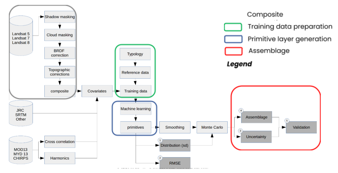
The RLCMS adopted a modular architecture outlined in Figure 1. The system is built on the GEE computational platform. The GEE is an online service that applies cloud computing and storage frameworks to geospatial datasets. The GEE archive contains a large amount of earth observation data. The platform enables scientists to perform calculations on large data series in parallel. The description of each module is given in the following sections.

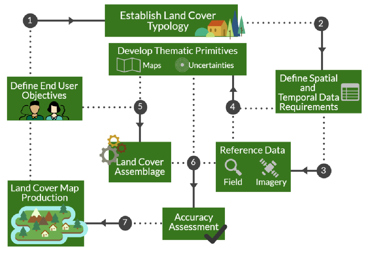
Figure 1: Regional Land Cover Monitoring System modular architecture

1.4.2 Defining end users objectives

During the consultation process, end users expressed the following main objectives for developing a regional land cover monitoring system:

Produce a regional, annually updated land cover map that will:

be based on consistent, transparent, contemporary, and defensible methods,

be accompanied by a robust accuracy assessment,
address most pressing regional business needs, and
address individual country needs where possible.

Provide easily accessible and user-friendly analysis tools and products. These will:

be optimized for integration with time-series analysis,
support multiple purposes and multi-users, and
be easily accessible and available to all countries and agencies.

1.4.3 Establishing land cover typology

After the objectives have been formulated and agreed upon, the next step is defining the land cover classes needed to produce the desired land cover map. The criteria to develop the land cover classes depend on the purpose of and the resources devoted to the mapping project. The regional land cover monitoring system requires robust land cover typologies and definitions. These are important for defining the map assemblage and reference data collection. A classification system, or typology, should be clear, precise, and based upon objective criteria. To guide the process of developing a land cover scheme, the following typology principles were established based on existing literature and group discussion (Faber et al. 2009, F.G.D. Committee 1977):

Stakeholder engagement: Stakeholders identify their needs as a basis for the typology,
Objective driven: A typology facilitates stakeholder objectives,
Simple: A typology is not more complicated than necessary to address stakeholder objectives,
Exhaustive: Each location on the map is represented in the typology,
Integrity among classes: Classes are mutually exclusive and have explicit class boundaries,
Consistent: The typology is consistent from one area of the map to another, and from one generation of land cover mapping to another to support trend monitoring,
Clear definitions: Map classes reflect measurable, diagnostic, biophysical features,
Differentiates land use from land cover: The typology separates land use and land cover themes,
Mappable: The typology is technologically and operationally feasible, for given budget and time constraints, and
Considers existing land cover schemes: Uses components of existing typologies whenever possible to maximize compatibility, shareability, and the use of available mapping technology, data, and applications.

To develop the shared land cover typology, the RLCMS uses the Land Cover Classification System (LCCS) and associated tool developed by FAO (Di Gregorio et al. 2016, Di Gregorio 2005, Di Gregorio and Jansen 1998). The LCCS presents a framework for precisely defining the land cover classes that users are interested in characterizing, such as mapping from remotely sensed imagery or inventorying from high resolution imagery. The LCCS assists users in systematically defining land cover categories from specific observable land cover characteristics or attributes, along with their spatial and temporal relationships. LCCS approach is used to determine the typology using biophysical elements that can be mapped and assembled into a final land cover map.

1.4.4 Defining Spatial and temporal data requirements

Available satellite data were reviewed by the RLCMS team to select appropriate data sets that would meet the design and production criteria of RLCMS. While choosing satellite data, RLCMS team considered the following criteria:

Data should be free to ensure sustainability,
Produced consistently to facilitate annual monitoring,
Moderate resolution useful for national and regional level assessment, and
Historical data availability for longer term change analysis.

While Landsat (Roy et al. 2014) and Sentinel 2 (Drusch et al. 2012) data fulfil all the first three criteria, Landsat data were chosen on the basis of availability of historical archive (Figure 2). In addition to satellite data, other contextual data such as elevation (Farr et al. 2007), infrastructure, river stream networks are used if available and suitable for specific primitives.

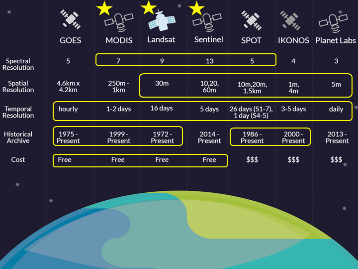
Figure 2: Launch and operational phase of different satellite images.

Algorithms were developed and implemented to pre-process Landsat data for atmospheric and terrain correction. The USGS Landsat 4, 5, 7, and 8 surface reflectance products are used in order to have a consistent time-series. The atmospherically corrected orthorectified surface reflectance data products are hosted in the Earth Engine data archive. Images from Landsat missions 4, 5 and 7 have been atmospherically corrected using LEDAPS (Masek et al. 2006, Schmidt et al. 2013, Vermote et al. 1997, Ju et al. 2012), and comes with band with a cloud, shadow, water and snow mask produced using CFMASK (Zhu et al. 2012), as well as a per-pixel saturation mask. Landsat 8 data have been atmospherically corrected using the Landsat Surface Reflectance Code (LaSRC) (Vermote et al. 2016, Holden et al. 2016, Roy et al. 2016) and also contains the data produced by CFMASK. Landsat 7 ETM+ for after the 2003 Scan Line Corrector failure were not included in the analysis as scan line effects were found to propagate through the data analysis into the final product. Discarding Landsat 7 left a gap for 2012, as Landsat 5 was decommissioned in May 2012, whereas Landsat 8 was launched in 2013. The 2012 primitives were created by temporal interpolation using the Whittaker smoothing algorithm.

Additional image pre-processing was applied since these images are subject to distortion as a result of sensor, solar, atmospheric, and topographic effects (Young et al. 2017). In order to produce reliable and consistent time series, it is important to account for these effects. We applied shadow and cloud removal, a bidirectional reflectance distribution function (BRDF) and topographic correction. We describe each in the following sections. Then we include the calculations and derivative list we used to create the full stack of Landsat derived covariates in the supervised classification model.

We mask clouds using the pixel-qa band and the Google cloudScore algorithm. Google's cloudScore algorithm uses the spectral and thermal properties of clouds to identify and remove pixels with cloud cover from the imagery. The algorithm identifies pixels that are bright and cold, then compares to the spectral properties of snow. The snowscore was also calculated using the Normalized Difference Snow Index (NDSI) to prevent snow from being masked. The algorithm calculates scaled cloud scores for the blue, all visible, near-infrared and short-wave infrared bands and then takes the minimum. The algorithm was described by (Chastain et al. 2019).

To remove cloud shadows, we used the Temporal Dark Outlier Mask (TDOM) algorithm (Housman et al in review) which identifies pixels that are dark in the infrared bands but are found to not always be dark in past and/or future observations. This is done by finding statistical outliers with respect to the sum of the infrared bands. Next, dark pixels were identified by using the sum of the infrared bands (NIR, SWIR1, and SWIR2). The pixel quality attributes generated from the CFMASK algorithm (pixel-qa band) was also used for shadow masking. The nadir view angles of the Landsat satellites cause directional reflection on the surface which can be described by the bidirectional reflectance distribution function (BRDF) (Roy et al. 2016, Roy et al. 2017, Lucht et al. 2000). We applied the method of Roy et al. (2016) to all images in the image collection.

Topographic correction is a radiometric process to account for illumination effects from slope, aspect, and elevation that can cause variations in reflectance values for similar features with different terrain positions (Colby 1991, Riano et al. 2003, Shepherd and Dymond 2003). We applied the Modified Sun-Canopy-Sensor Topographic Correction method as described by Soenen and colleagues (2005). The algorithm combines the sun-canopy-sensor (SCS) (Gu et al. 1998) with a semiempirical moderator (C) to account for diffuse radiation (Justice et al. 1981, Smith et al. 1980, Teillet et al. 1982). The model contains physically based corrections that preserve the sun-canopy sensor geometry (SCS, SCS+C) while adjusting for terrain.

1.4.5 Reference Data

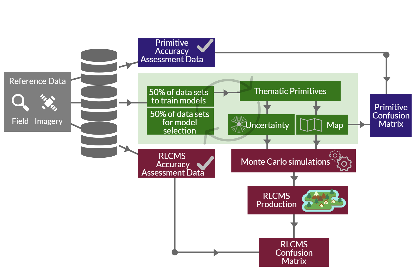
Quality assured reference data is critical for RLCMS development and assessment. Reference data are collected from the field through national partners. Additional reference data are obtained from high resolution satellite images using Collect Earth desktop or Collect Earth online software. Reference data are divided into three lots. These were used for (i) primitive accuracy assessment, (ii) primitive development and (iii) accuracy assessment of final land cover maps to produce a confusion/error matrix, as shown in Figure 3.

1.4.6 Develop thematic primitives

The primitives are mappable biophysical elements that can be used by themselves or combined to define a class. The primitives represent raw information needed to make decisions in a dichotomous key for land cover typing. For example, to classify a location as “deciduous forest” (Figure 4), one may need to know the “percent canopy closure”, “average canopy height” and “phenology”. Percent canopy closure, expressed as a geographic raster dataset, is a land cover primitive. This approach is not only highly suitable to remotely sensed raster datasets, but also highly flexible in terms being able to meet the needs of multiple stakeholders. For example, different countries may use different thresholds for canopy cover percent while defining forest.

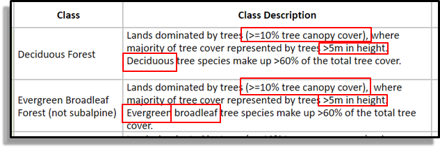
Figure 4: These primitive layers are reassembled to create a final land cover map product according to a decision logic that results in land cover classes corresponding to the desired land cover typology.

1.4.7 Land cover assemblage

Monte Carlo analysis is used when assembling primitives into land cover classes. Primitive maps with their associated uncertainties (standard deviation for percent cover layers, and probabilities for the thematic layer) are first developed as described above and assembled according to a decision logic that results in land cover classes corresponding to the developed typology (see Figure 5, for example). Instead of assigning land cover classes according to whether pixel values pass defined thresholds (e.g. 10% canopy cover, deciduous, etc.), the distribution of probable values associated with the pixel values is sampled many times and the modal or majority prediction is then used in defining the land cover class.

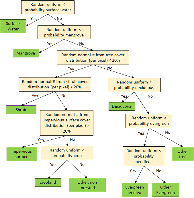
Figure 5: Example of assemblage decision tree logic example

In comparison with alternative probabilistic classification methodologies, such as Bayesian networks or fuzzy logic, Monte Carlo sampling over deterministic decision trees enables end-users to construct bifurcating decision trees by posing yes/no land cover-related questions. Because the primitives are probabilistic, sampling from them independently within the group-designed decision trees and collecting aggregate statistics enables retention of as much of the input data's uncertainty in the final products as possible. Although a Bayesian network approach may provide a clearer uncertainty propagation scheme to those familiar with probabilistic mathematics, the Monte Carlo methodology is considered more easily and widely understood and therefore more appropriate.

The procedures used in developing the RLCMS allow for specific primitive layers to be prioritized in the decision logic to increase accuracy in relation to themes of interest. This enables users to restructure the assemblage to fit specific needs if standard RLCMS maps are not appropriate. Depending on reference data availability, the typology can also be modified with the accuracy assessment and confusion/error matrix updating accordingly.

1.4.8 Accuracy assessment

A standard accuracy assessment method for remote sensing-based classification will be adopted (Olofsson et al. 2014). Two levels of assessment will be conducted:

Accuracy assessment of individual primitives and
Accuracy assessment of the final map.

The following steps will be used for the accuracy assessment:

Visual interpretation: Classification results will be visually investigated to identify any gross and systematic error. Based on the feedback of this investigation, appropriate measures will be taken to improve the classification. The output will be also reviewed by participants from partner organisations with knowledge of land cover distribution of the country.
Quantitative accuracy assessment: We will use randomly selected, independent, reference data that was generated from a probability sample for accuracy assessment. This data will be used to generate error matrices for each primitive separately and for the final land cover map.

1.4.9 Computational platform

The regional land cover monitoring system is built on the GEE computational platform. The GEE is an online service that applies cloud computing and storage frameworks to geospatial datasets (Gorelick et al. 2017). The archive contains a large amount of earth observation data. The platform enables users to perform calculations on large data series in parallel.

1.4.10 Challenges and risks

Once the RLCMS has been refined such that we have map products with good accuracy and confidence levels, the system will make it easier for users to generate quality land cover maps and statistics. The system applications are user-friendly. However, there are still some associated risks we should make a note of, including access policies to remote sensing images, the Google Earth Engine computational platform, and reference data. Further the system creates maps at a 30 m resolution, which might miss land cover patterns that occur at a finer spatial resolution. We describe each of these risks in further detail below.

RLCMS relies heavily on data from the Landsat program. If there are any policy changes that will impact the continuity of Landsat 8 or 9 we will note to adapt the system to generate future land cover map products. We are also taking advantage of the freely available Google Earth Engine platform. If at some point Google changes the accessibility of the platform to a commercial product, we will have to reassess the service costs.

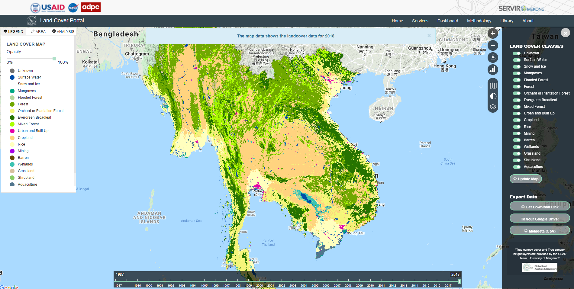
1.5 Example of RLCMS implementation in SERVIR Mekong

The first version of the RLCMS approach has been implemented in SERVIR Mekong covering 5 Lower Mekong countries (Myanmar, Thailand, Lao PDR, Cambodia, and Vietnam) plus a defined buffer. The system is now available at SERVIR Mekong RLCMS portal at https://www.landcovermapping.org/en/landcover/

1.6 Expansion to SERVIR HKH

With successful experience in the Mekong Region, SERVIR HKH and SERVIR Mekong began collaborating to implement the system for Hindu Kush Himalayan Countries. A regional workshop was organized in Bangkok, and several country workshops have been organized in Nepal, Afghanistan and Myanmar. The first version of the national land cover monitoring system (NLCMS) for forest resources assessment for Myanmar was submitted to the Forest Department of Myanmar. The first round of reference data collection for Nepal in collaboration with Forest Resources Training Center (FRTC) is completed and further enhancement of the system has been done in cooperation with USFS (algorithm enhancement and implementation) and FAO (online reference data collection application and integration into SEPAL).

Overall Workflow for National Land Cover Monitoring System

Broadly, the overall method can be divided into four major steps (Figure 7). They are;

Composite preparation:

It involves image pre-processing such as shadow and cloud masking, BRDF and topographic correction. Available Landsat 5, 7 and 8 images are used for the composites preparation.

Training data preparation: It involves identifying typology for the particular country on the basis of which reference data are being collected. The reference data are segregated into training data and validation data. The training data are sampled to get information/data at pixel level. Several covariates are used in this step.
Primitive layers generation:

The data obtained from training data sampling are used by the classifier to generate primitive layers. These primitive layers represent probability of a certain biophysical feature existing within that pixel. Assessment of primitive layers are also done.

Assemblage to create final land cover map:

In this step, the decision tree is developed based on user specified thresholds. The thresholds are determined on the basis of visual assessment and primitive assessment plots.

GEE Code repository

Go to the following path; then you will get an interface as in Figure 8.

https://code.earthengine.google.com/?accept_repo=users/khanalnishant/RLCMS

On the left side of the page, you will see scripts, Doc and Assets (Figure 8).
Go to the repository, users/khanalnishant/RLCMS where you can see two folders namely MainScripts and SupportScripts
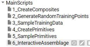
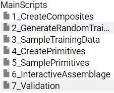
In the MainScripts folder, there are six files (Figure 9). They are;

1_CreateComposites,

2_GenerateRandomTrainingPoints,

3_SampleTrainingData,

4_CreatePrimitives,

5_SamplePrimitives and

6_InteractiveAssemblage

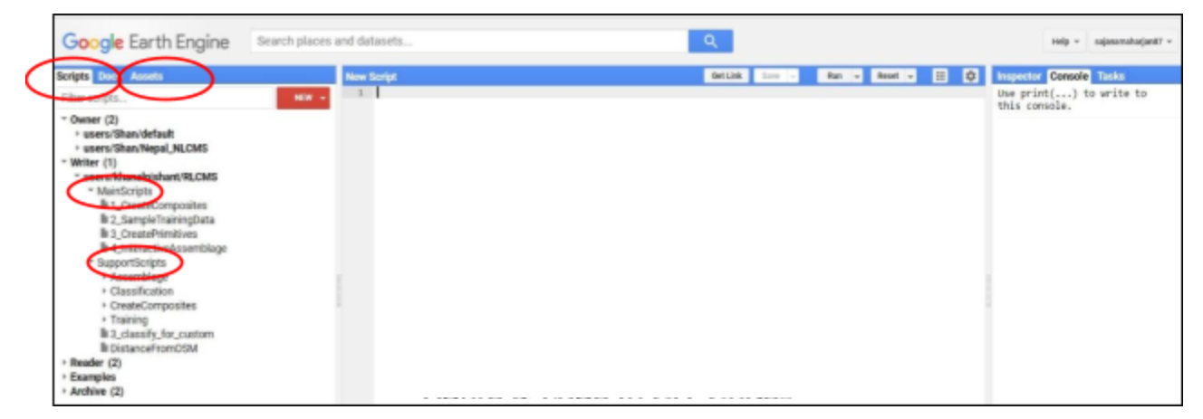
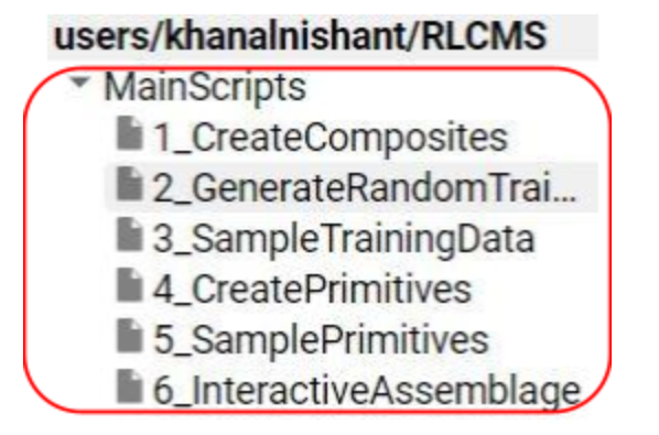
Figure 9

Create folder in the Assets and upload your study area in it

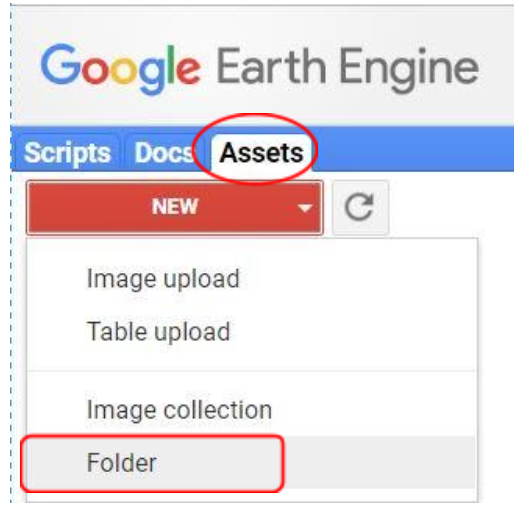
Go to the Assets Tab, click on it. Then you will get a list to choose, click on Folder to create a new folder and name it as Bangladesh_Training (Figure 10).
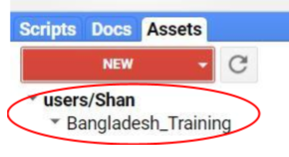
You will see a folder in your repository as shown in Figure 11.

In order to upload your study area, first make sure your boundary is in WGS 1984 (geographic coordinate system), and zip the file.
Go to the Assets, click on it then click on the Table upload (Figure 12).
You will see a window pop out as shown in Figure 13 where you need to select the path of your Zip file. Also, need to give the path for the file where you want to save it. For example, in this case, we want to save it in Bangladesh_Training folder (See Figure 13). Then click ok.
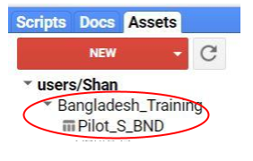
You can check in the Assets whether it is being uploaded or not (Figure 14).

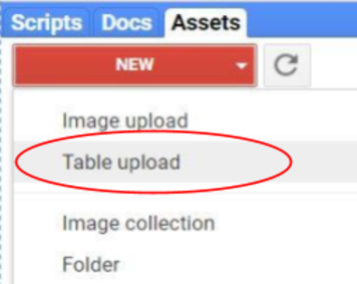
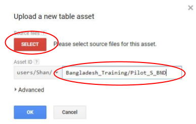
Figure 13

Create Image Collection in the Assets

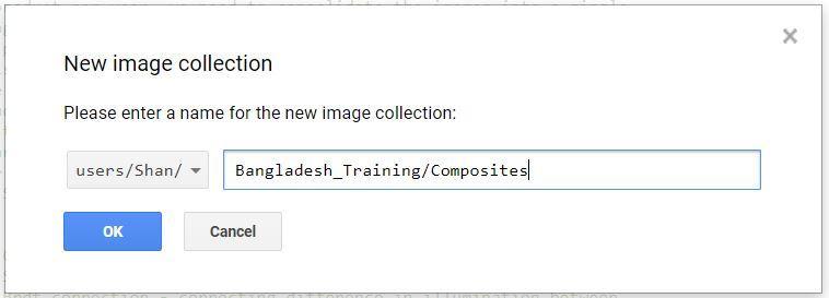
Go to the Assets, click on it then click on Image collection (Figure 15).
Give the path where you want to create image collection. In this case, we want to create it in Bangladesh_Training and give it the name as Composites (Figure 16). Then click ok.

You can check the created image collection in the folder of your Assets (Figure 17).

Create Composites

In order to create composite for your study, click on 1_CreateComposites file. There are the scripts for creating composites. In the scripts, you may need to change some variables to make compatible as per your needs. The variables that users can/should change to tune the result to their study area are;

1. boundary - the asset containing boundary of the area of study. It is better to use a buffered region so that it can be clipped to the actual area of interest at the end (Figure 18).

2. year – mention the year for which to prepare composite (Figure 18).

3. season - the season for which to prepare composite. This should be first set on the helper script. If exporting yearly composite, the values should be 'all' (Figure 18).

4. maxCloudCover - the maximum cloud cover percentage for an image to be considered for analysis (Figure 18).

5. exportScale - the spatial resolution of exported composite (Figure 18).

6. exportPath - the image collection id where to export composite (Figure 18).

To get the path of your uploaded file (boundary of study area), go to Assets, then to your folder, click on the file (Pilot_S_BND), a window will pop out as shown in Figure 19.
Copy the Table ID and paste it in the script line no. 77.
In the export path, you need to replace with your path, for this, go to Assets, click on Composites, a window will pop out as shown in Figure 20.
Copy the ImageCollection ID and paste it in the script line no. 82.
Now, you can run the script, the run button is at the top of the GEE interface (Figure 21).

Once you run, go to the task button, click on it. You will see a file on it.
Click on run button to export it (Figure 22). After it you will get a window as shown in Figure 23, make sure the path where you want to export it, and cell size. Then click on the run button.
Then, you can find the exported composites in your image collection.

Preparation of Training Samples

Training data may be already available from your department. However, the data may not be sufficient for the land cover classification. In such case, we can use collect earth tool developed by FAO which is a desktop version or collect earth online developed by SERVIR - a joint NASA and USAID program in partnership with regional technical organizations around the world - and the FAO as a tool for use in projects that require land cover and/or land use reference data.

In order to perform classification, we need to rely on the data obtained from remote sensing images as well other sources. These data that we use during classification are called covariates which are derived using our training data. In this script, we will extract these covariate dataset on the pixel where our reference points (which are actually our "known" points) are so that they will be used to train a classifier which is actually predicting class of other pixels (which are actually our unknown points).

For this, go to the script ‘page 3_SampleTrainingData’ (Figure 24).

In order to sample training data the variables that users can/should change are

1. boundary - This should contain the boundary of your study area (Figure 26: script line no. 49). To get the path of your study area follow the step mentioned in chapter 6, Figure 19.

2. repository - The repository that contains the composites required ( this is the folder that contains your 'composites' Image collection) (Figure 26: script line no. 50). To get the path, follow the step mentioned in chapter 6, Figure 20.

3. trainingData - this should be the table that contains reference points of your study area (Figure 26, script line no. 51). Here you need to give the path of your data.

NOTE: the dataset needs to have at least two columns one containing the information on land class (primitive level) at the point and another containing the information on the year that in represents. An example is given in Figure 25.

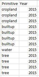
4. inputLandClass - this should contain the name of column that contains the primitive level information (Figure 26, script line no. 54)

5. inputYearClass - this should contain the name of column that contains the year information (Figure 26, script line no. 55)

6. sampleScale - (optional) this controls the scale at which the image is sampled. Its best to have it set the same as the resolution of your composite (Figure 26, script line no. 57)

7. exportId - (optional) the full id of target asset for export if exporting to asset. This can be changed later during export (Figure 26, script line no. 58). Follow chapter 5 Figure 16 and 17.

8. startYear - (optional) the year from which (inclusive) to start sampling the training data (Figure 26, script line no. 59)

9. endYear - (optional) the year till which (inclusive) to start sampling the training data (Figure 26, script line no. 60)

Once you change the variables, you can run the script clicking on the run button which is at the top of the GEE interface (Figure 21).
After the script is run, initiate the export task by going to the "Tasks" tab and click on the run button (Figure 22 and Figure 23).

Create Primitives

After reference points are being sampled, we need to create probability layers that will eventually feed into our assemblage logic. We will use random forest classifier to create primitive layers with output mode set as probability. Since the classification will be probability of a certain biophysical feature existing within that pixel, we will perform classification using only two classes;

1. Class that specifies that a certain feature exists

2. Class that specifies that said feature does not exist. For example, if we want to generate a tree cover primitive, we will set points that symbolize tree cover as class 1 and other points such as built up, rivers, etc as class 0.

For this, go to the script ‘4_CreatePrimitives’ (Figure 27).

In order to create primitive layers, the variables that users can/should change are

1. boundary - This should contain the boundary of your study area (Figure 28: script line no. 44). To get the path of your study area follow the step mentioned in chapter 6, Figure 19.

2. repository - this is the image collection that contains the composites (Figure 28: script line no. 45). To get the path, follow the step mentioned in chapter 6, Figure 20.

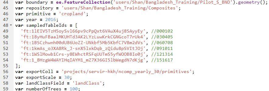
3. primitive - it is the name of the primitive (as in reference data) which we want to prepare primitive layer for (Figure 28 is for cropland, script line no. 46).

4. year - this is the year for which we want to produce the primitive layer (Figure 28, script line no. 47).

5. sampledTableId - this should contain the asset Id or fusion table id (starting with a "ft:" if its a fusion table) for the sampled table (Figure 28, script line no. 48).

6. landClassField - this should contain the name of column that contains the primitive level information (Fig 28, script line no. 58)

7. exportScale - this is the spatial resolution of the export layer (Fig 28, script line no. 57)

8. numberOfTrees - (optional) the number of trees or iteration used by random forest (Fig 28, script line no. 59)

Once you change the variables, you can run the script clicking on the run button which is at the top of the GEE interface (Figure 21).
After the script is run, initiate the export task by going to the "Tasks" tab and click on the run button (Figure 22 and Figure 23).

Note that there will be multiple exports for each year

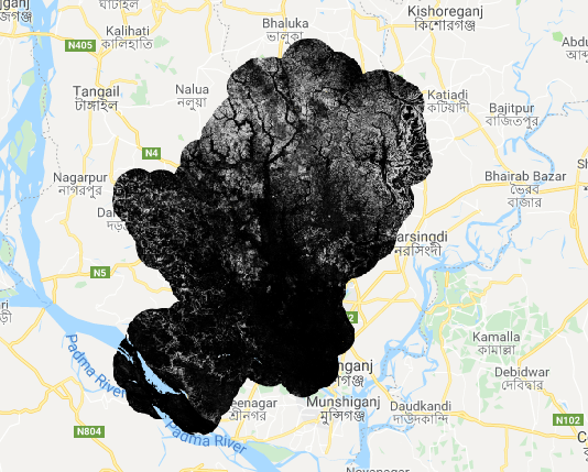
Figure 29 Tree Primitive example for 2015

Assessment of Primitives

We have produced several primitive layers to support our development of land cover maps. However, at this stage, we do not know the quality of these primitive layers. Therefore, we will check the quality of these primitive layers using validation points. We do this by plotting probability distribution of points throughout a certain primitive over all the years. This gives the information on the distribution of probabilities throughout the points that are supposed to be of same class vs those that are supposed to be of different class.

For this, go to the script ‘5_SamplePrimitives’ (Figure 30).

In order to assess primitive layers, the variables that users can/should change are

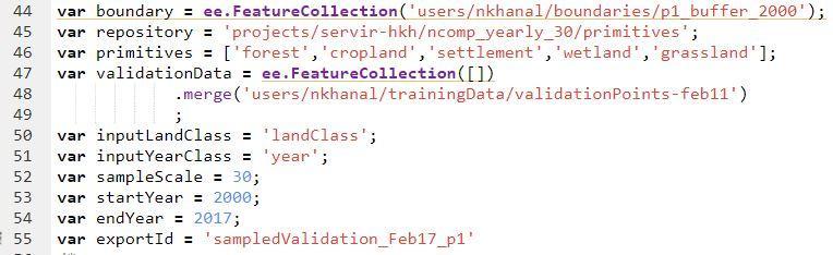
1. boundary - This should contain the boundary of your study area (Figure 31: script line no. 44). To get the path of your study area follow the step mentioned in chapter 6, Figure 19.

2. repository - The repository that contains the composites required ( this is the folder that contains your 'primitives' Image collection) (Figure 31: script line no. 45). You need to give your repository path.

3. validationData - This should be the table that contains validation points (Figure 31: script line no. 47). You need to give your validation data path.

NOTE : The dataset needs to have at least two columns one containing the information on land class (primitive level) at the point and another containing the information on the year that in represents

4. inputLandClass - this should contain the name of column that contains the primitive level information (Figure 31: script line no. 50).

5. inputYearClass - this should contain the name of column that contains the year information (Figure 31: script line no. 51).

6. sampleScale - (optional) this controls the scale at which the image is sampled. Its best to have it set the same as the resolution of your composite (Figure 31: script line no. 52).

7. startYear- the year from which (inclusive) to start sampling the validation data (Figure 31, script line no. 53)

8. endYear- the year till which (inclusive) to start sampling the validation data (Figure 31, script line no. 54)

9. exportId - (optional) the full id of target asset for export if exporting to asset. This can be changed later during export (Figure 31: script line no. 55).

Once you change the variables, you can run the script clicking on the run button which is at the top of the GEE interface (Figure 21).
After the script is run, initiate the export task by going to the "Tasks" tab and click on the run button (Figure 22 and Figure 23).

Note that if your reference dataset is too large and you consistently get computation or memory limit or other errors, you may want to break it down and run the script with subsets of the reference data.

Figure 32 is showing Probability Distribution Plots for primitive assessment

$C:\Users\nkhanal\AppData\Local\Microsoft\Windows\INetCache\Content.Word\Builtup.png$

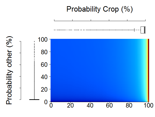
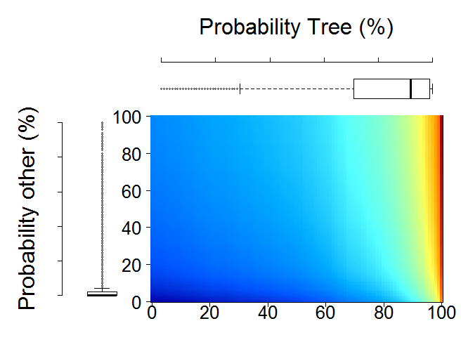
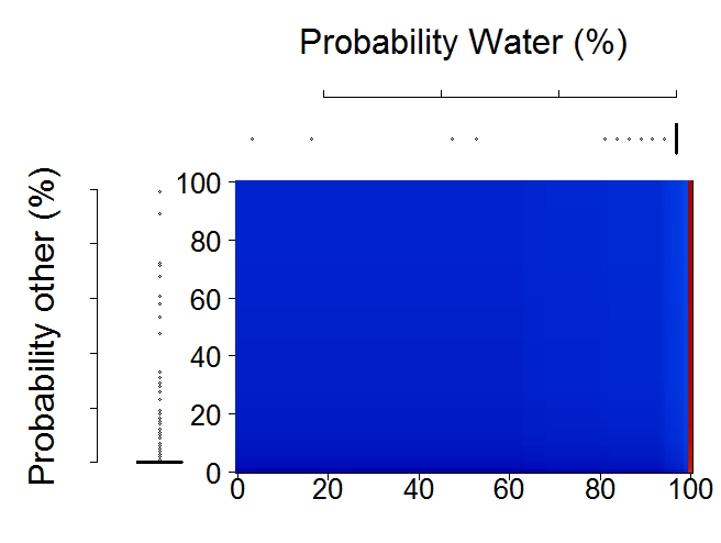
Figure 32 Probability Distribution Plots for primitive assessment

Interactive Assemblage

Once we have satisfactory primitives we will run them through assembler to obtain a land cover map. The assembler prepares a decision tree based on user specified thresholds which can be determined based on visual assessment as well as primitive assessment plots. The order of primitives in the list denotes the order in which primitives are placed in the decision tree with the first primitive placed on the top and so forth. This basically means that if a pixel has high probability on two primitives (according to the specified threshold) the final class will be based on the primitive that is higher up on the decision tree.

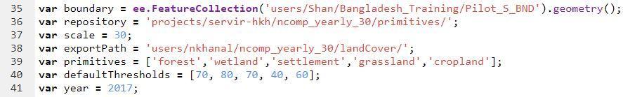
For this, go to the script ‘6_InteractiveAssemblage’ (Figure 33).

For this step, the users can/should change the following parameters;

1. boundary - This should contain the boundary of your study area (Figure 34: script line no. 35). To get the path of your study area follow the step mentioned in chapter 5, Figure 13.

2. repository - The repository that contains the stack of primitives required (Figure 34: script line no. 36). You need to give your repository path that consists of primitives stack.

3. scale - The spatial resolution of the resulting landCover (Figure 34: script line no. 37).

4. exportPath - The path in which to export the resulting landcover (Figure 34: script line no. 38).

5. primitives - The list of primitives to include in the assembler (Figure 34: script line no. 39).

6. defaultThresholds - (optional) The default thresholds that the interface initiates with. It can be changed in the user interface later. This should be in line with the list of primitives. (Figure 34: script line no. 40).

7. year - The default year to load into the interface (Figure 34: script line no. 44). It can be changed

in the interface.

Once you change the variables, you can run the script clicking on the run button which is at the top of the GEE interface (Figure 21).
After the script is run, initiate the export task by going to the "Tasks" tab and click on the run button (Figure 22 and Figure 23).
Figure 35 is showing the final land cover map.

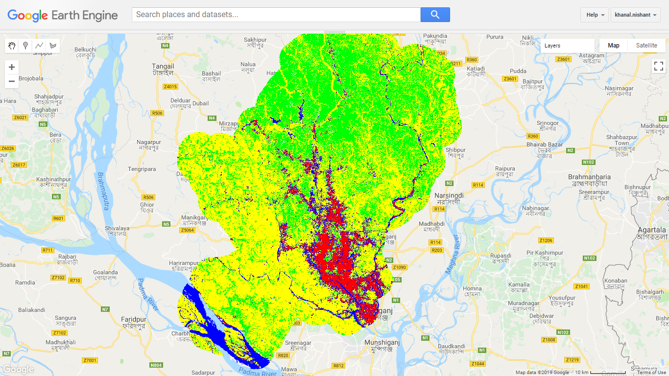
Figure 35: Land cover Map in Google Earth Engine

Validation

Once we have a set of land cover maps, we need to check quality of the maps. For this, we do accuracy assessment of the maps. We use a set of data separated for validation purposes which were not used in training the model.

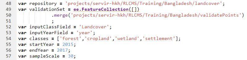
For this, go to the script ‘7_Validation’ (Figure 36)

The variables that users can/should change are

1. repository - The repository that contains the land cover maps required. You need to give your repository path that consists of land cover maps (Figure 37: script line no. 48).

2. validationData - This should be the table that contains validation points. Give the path of your validation data (Figure 37: script line no. 49).

NOTE : the dataset needs to have at least two columns one containing the information on land class at the point and another containing the information on the year that in represents

3. inputClassField - This should contain the name of column that contains the land class information (Figure 37: script line no. 52).

4. inputYearField - This should contain the name of column that contains the year information (Figure 37: script line no. 53).

5. classes - Since the validation points will have classes information as a text, we need to convert them to their numeric representative as the land cover maps have them as numbers. Therefore, this should be a list of classes in order of their values ranging from 1 to number of classes (Figure 37: script line no. 54).

6. startYear - The year from which to perform accuracy assessment. (inclusive) (Figure 37: script line no. 55).

7. endYear - The year to which to perform accuracy assessment. (inclusive) (Figure 37: script line no. 56).

8. sampleScale - (optional) This controls the scale at which the image is sampled. It is best to have it set the same as the resolution of your composite (Figure 37: script line no. 57).

Once you change the variables, you can run the script clicking on the run button which is at the top of the GEE interface (Figure 21).
After the script is run, view the accuracy statistics by going to the "Console" tab (Figure 38).

References:

A. Di Gregorio, et al., Land cover classification system: Classification concepts. software version 3 (2016).

A. Di Gregorio, L. J. Jansen, Land cover classification system (lccs): classification concepts and user manual, FAO, Rome (1998).

A. Di Gregorio, Land cover classification system: classification concepts and user manual: LCCS, volume 8, Food & Agriculture Org., 2005.

C. E. Holden, C. E. Woodcock, An analysis of landsat 7 and landsat 8 underflight data and the implications for time series investigations, Remote Sensing of Environment 185 (2016) 16–36.

C. O. Justice, S. W. Wharton, B. Holben, Application of digital terrain data to quantify and reduce the topographic effect on landsat data, International Journal of Remote Sensing 2 (1981) 213–230.

D. Faber-Langendoen, D. L. Tart, R. H. Crawford, Contours of the revised us national vegetation classification 693 standard, The Bulletin of the Ecological Society of America 90 (2009) 87–93.

D. Gu, A. Gillespie, Topographic normalization of Landsat TM images of forest based on subpixel sun–canopy–sensor geometry, Remote sensing of Environment 64 (1998) 166–175.

D. P. Roy, J. Li, H. K. Zhang, L. Yan, H. Huang, Z. Li, Examination of sentinel-2a multi-spectral instrument (msi) reflectance anisotropy and the suitability of a general method to normalize msi reflectance to nadir brdf adjusted reflectance, Remote Sensing of Environment 199 (2017) 25–38.

D. P. Roy, M. Wulder, T. R. Loveland, C. Woodcock, R. Allen, M. Anderson, D. Helder, J. Irons, D. Johnson, R. Kennedy, et al., Landsat-8: Science and product vision for terrestrial global change research, Remote Sensing of Environment 145 (2014) 154–172.

D. P. Roy, V. Kovalskyy, H. Zhang, E. F. Vermote, L. Yan, S. Kumar, A. Egorov, Characterization of landsat 7 to landsat-8 reflective wavelength and normalized difference vegetation index continuity, Remote Sensing of Environment 185 (2016) 57–70.

Drusch, M., Del Bello, U., Carlier, S., Colin, O., Fernandez, V., Gascon, F., ... & Meygret, A. (2012). Sentinel-2: ESA's optical high-resolution mission for GMES operational services. Remote Sensing of Environment, 120, 25-36.

E. F. Vermote, D. Tanre, J. L. Deuze, M. Herman, J.-J. Morcette, Second simulation of the satellite signal in the solar spectrum, 6s: An overview, IEEE transactions on geoscience and remote sensing 35 (1997) 675–686.

E. Vermote, C. Justice, M. Claverie, B. Franch, Preliminary analysis of the performance of the Landsat 8/OLI land surface reflectance product, Remote Sensing of Environment 185 (2016) 46–56.

F. G. D. Committee, et al., Vegetation subcommittee. vegetation classification standard. fgdcstd-005. federal 695 geographic data committee, US Geological Survey, Reston, Virginia, USA. [Available online: http://www.fgdc.696gov/standards/documents/standards/vegetation/vegclass.pdf] (1977)

G. Schmidt, C. Jenkerson, J. Masek, E. Vermote, F. Gao, Landsat ecosystem disturbance adaptive processing system (LEDAPS) algorithm description, Technical Report, US Geological Survey, 2013.

Gorelick, N., Hancher, M., Dixon, M., Ilyushchenko, S., Thau, D., & Moore, R. (2017). Google Earth Engine: Planetary-scale geospatial analysis for everyone. Remote Sensing of Environment, 202, 18-27.

J. D. Colby, Topographic normalization in rugged terrain, Photogrammetric Engineering and Remote Sensing 57 (1991) 531–537.

J. G. Masek, E. F. Vermote, N. E. Saleous, R. Wolfe, F. G. Hall, K. F. Huemmrich, F. Gao, J. Kutler, T.-K. Lim, A Landsat surface reflectance dataset for north america, 1990-2000, IEEE Geoscience and Remote Sensing Letters 3 (2006) 68–72.

J. Ju, D. P. Roy, E. Vermote, J. Masek, V. Kovalskyy, Continental-scale validation of modis-based and ledaps Landsat ETM+ atmospheric correction methods, Remote Sensing of Environment 122 (2012) 175–184.

J. Smith, T. L. Lin, K. Ranson, et al., The Lambertian assumption and Landsat data, Photogrammetric Engineering and Remote Sensing 46 (1980) 1183–1189.

Lucht, W., & Roujean, J. L. (2000). Considerations in the parametric modeling of BRDF and albedo from multiangular satellite sensor observations. Remote Sensing Reviews, 18(2-4), 343-379.

N. E. Young, R. S. Anderson, S. M. Chignell, A. G. Vorster, R. Lawrence, P. H. Evangelista, A survival guide to Landsat preprocessing, Ecology 98 (2017) 920–932.

Olofsson, P., Foody, G. M., Herold, M., Stehman, S. V., Woodcock, C. E., & Wulder, M. A. (2014). Good practices for estimating area and assessing accuracy of land change. Remote Sensing of Environment, 148, 42-57.

P. Teillet, B. Guindon, D. Goodenough, On the slope-aspect correction of multispectral scanner data, Canadian Journal of Remote Sensing 8 (1982) 84–106.

R. Chastain, I. Housman, J. Goldstein, M. Finco, K. Tenneson, Empirical cross sensor comparison of sentinel-2a and 2b MSI, Landsat-8 oli, and landsat-7 etm+ top of atmosphere spectral characteristics over the conterminous united states, Remote Sensing of Environment 221 (2019) 274–285.

S. A. Soenen, D. R. Peddle, C. A. Coburn, Scs+ c: A modified sun-canopy-sensor topographic correction in forested terrain, IEEE Transactions on geoscience and remote sensing 43 (2005) 2148–2159.

Shepherd, J. Dymond, Correcting satellite imagery for the variance of reflectance and illumination with topography, International Journal of Remote Sensing 24 (2003) 3503–3514.

T. G. Farr, P. A. Rosen, E. Caro, R. Crippen, R. Duren, S. Hensley, M. Kobrick, M. Paller, E. Rodriguez, L. Roth, et al., The shuttle radar topography mission, Reviews of geophysics 45 (2007).

W. Lucht, C. B. Schaaf, A. H. Strahler, An algorithm for the retrieval of albedo from space using semiempirical brdf models, IEEE Transactions on Geoscience and Remote Sensing 38 (2000) 977–998.

Z. Zhu, C. E. Woodcock, Object-based cloud and cloud shadow detection in landsat imagery, Remote Sensing of Environment 118 (2012) 83–94.