Homework 3: The Cloud, Matrices, and Arrays

Due March 18, 2017 by 10pm

For this assignment, we will focus on array and matrix data.  An array is a multidimensional set of values of the same type, and we’ll often encode matrices within arrays.  Arrays are going to be incredibly useful for multidimensional data, for images, for matrices, for representing documents, and for machine learning training data.  (We’ll see the last aspect in a future assignment.)

As part of this assignment, you’ll also build upon HW2 and execute a computation in Elastic MapReduce on Amazon.  Depending on your skill level, you can use a shared server we’ve set up (with the caveat that you should *start early* because it will be in heavy contention) or set your own server up (with the caveat that you will need to get credits from Amazon or spend a few dollars).

Step 1. Set up Spark on the Amazon Cloud

The first part of your homework will involve connecting to Jupyter on Amazon Elastic MapReduce (EMR) on the Cloud.  Here you have two options:

1. For most users (especially those intending to do a project later in the term):
   set up your own Amazon AWS Educate account and server.
2. For novice users:  connect to the CIS 700-003 Shared Jupyter Server.  Note that this may be shared with many more users, and performance will be less dependable.

Step 2. Use Spark on Amazon EMR

Let’s start by downloading the data files for this assignment, both into your Docker instance and into JupyterHub.  

Step 2.1. Download the Repo into Your Docker Container

Go to your operating system’s Terminal or Command Prompt.  Go to ~/jupyter.  Run the command:

git clone https://bitbucket.org/pennbigdataanalytics/hw3.git

You’ll come back to this soon.

Step 2.2. Download the Repo into Your EMR Jupyter/JupterHub Server

Now go to Jupyter on Amazon in your browser (the shared JupyterHub is at http://ec2-54-85-56-114.compute-1.amazonaws.com:8000; if you set up your own server then it is as in the end of this document), open a new Terminal there (click the “New” dropdown in the top right and select “Terminal”) and run the following to clone the HW3 repository:

git clone https://bitbucket.org/pennbigdataanalytics/hw3.git

Now in JupyterHub, go into hw3 and create a new Python 3 Notebook called Spark.  Type in the following:

from emrspark import *

from pyspark.sql.types import *
import pyspark.sql.functions as F

conf.set("fs.s3n.awsAccessKeyId","**")

conf.set("fs.s3n.awsSecretAccessKey","**")

spark = SparkSession.builder.config(conf=conf).appName('Graph HW3').getOrCreate()

Where, for the AWS access key and secret key above, replace the “**”s with the values posted to Piazza.  (Please don’t share our credentials with others!)

Step 2.3. Transitive Closure over the Stack Overflow Network

In the previous assignment, you had built several primitives, including breadth-first search, to compute over the Stack Overflow social graph.  Some of your computations were limited by the amount of computational resources available.  We will now try to explore the broader graph.

Step 2.3.1. Loading the Data

The three source files (sx-stackoverflow-a2q.txt, sx-stackoverflow-c2q.txt, sx-stackoverflow-c2a.txt) from Homework 2 are loaded onto Amazon S3 (Amazon’s “cloud disk” service) in the path s3n://upenn-bigdataanalytics/data.  As with Homework 2 Step 2.3, you will combine them into a unified graph_sdf.  

You will need to load each file from Amazon in a different way than before.  (1) We’ll be reading off Amazon’s S3 service and (2) we will try to do the parsing into fields inline with the read.  You can use a command such as:

my_sdf = spark.read.format("com.databricks.spark.csv").option("delimiter", ' ') \

  .load("s3n://upenn-bigdataanalytics/data/myfile.txt")

to load the space-delimited file myfile.txt into a Spark DataFrame with columns named _c0, _c1, etc. (Downloading these files may take a while, so don’t worry). See if you can further add a function call (e.g., to selectExpr()) to rename the first two columns to from_node and to_node, to convert these to integers, and to drop the third column.  Union everything together (and remove duplicates) to create graph_sdf with all data.  Note that .union() in Spark is an alias for .unionAll().

Hints: For early testing of your solutions to Step 2, you should probably just load one of these files (eg sx-stackoverflow-a2q.txt) into graph_sdf to validate your solutions.  Later go back, add the contents of the other files to graph_sdf, and re-run your solutions.  Make sure you rerun your code with the full graph_sdf before submitting.

Step 2.3.2. Transitive Closure of the Graph

Now we would like to do the following: given a set of nodes, compute the set of all nodes reachable from these nodes.  This can be obtained via a type of transitive closure computation.

Define a function transitive_closure(graph_sdf, origins_sdf, depth) that returns a Spark DataFrame.

The result should be the set of all nodes from the input graph_sdf that are reachable via graph edges from the set of origins_sdf, in at most depth iterations (hops).  Both origins_sdf and the returned result should be DataFrames with a single attribute called node.  

You should treat the edges in the graph_sdf as directed edges!  You should iterate until you have either hit the maximum depth or the set of newly discovered (frontier) nodes is empty.

Hints: this resembles your BFS algorithm from HW2, but you should take advantage of the opportunities to optimize.  Both the graph and the various node sets can easily have duplicates; you should make heavy use of duplicate removal (and repartition and cache) since you are only computing the set of reachable nodes. Also, to quickly check whether a DataFrame is empty, you can use something similar to the following:

def sdf_is_empty(sdf):

    try:

        sdf.take(1)

        return False

    except:

        return True

If you are using the shared JupyterHub server, please be courteous to your fellow students.  The JupyterHub server is a shared resource.  Whenever you are done with this part of the assignment, or wish to take a break, please shut down your personal Jupyter Notebook instance, as per the instructions.

Step 3. PageRank with Matrices

[Note: if you can’t read the equations below due to a bug in GDoc, click on the link to the lower right that says: Document doesn't display correctly? See the original Google Doc.  Alternatively, if you right-click on the broken image and choose “Open Image in New Tab” you’ll see it.]

For this part of the assignment, we can go back to our Jupyter instance on Docker, since we’ll be doing matrix operations in Numpy/Scipy.  In your Jupyter instance (localhost:8888) create a new Python 3 notebook called PageRank.  [If you set up your own private EMR server you can use it as well.]

Recall that PageRank can be modeled using matrix operations as follows.  Let M be a weight transfer matrix in which:

                if page i is pointed to by page j and page j has nj outgoing links                              = 0              otherwise

And define a dampening factor 𝛂 = 0.85 and a corresponding 𝜷 = 1 - 𝛂.  Initialize the PageRank vector

(i.e., a matrix with m rows by 1 column, filled with ones).  Then we can compute the PageRank PR for each iteration as:

Step 3.1. Download a Web Graph

Recall from Homework 2 that you were given a Jupyter Notebook called Retrieve.ipynb, which downloaded a series of zipped text files from Stanford SNAP and decompressed them.  Adapt that code to download:  https://snap.stanford.edu/data/web-NotreDame.txt.gz

which is a reasonably sized Web crawl done by Notre Dame University, and to extract it into web-NotreDame.txt.  Run the program to acquire your Web graph.

Step 3.2. Load the Notre Dame Web Graph into a Matrix

Next, write Python code to take the data from web-NotreDame.txt, read and parse the rows in a Pandas DataFrame (not a Spark DataFrame!).  Restrict the node IDs to values less than 10,000. Create a weight transfer matrix M corresponding to the Web graph, with edges whose weights are scaled as per the PageRank definition of a weight transfer matrix.  This will form an input into your PageRank algorithm.  Note that the dataset already includes node IDs that go from 0 .. m, so you can directly use the node IDs as indices in your matrix.  You should not use for loops, and instead, use the DataFrame and array functions that Pandas and NumPy provide as they are much more efficient.

Hints: If you use read_csv, you may need to look at the sep and skiprows options.  Also take a look at the raw data and make sure you know how many rows don’t contain data, and how the items are separated.  When building M, you may need to build some “auxiliary” data structures to speed up performance, e.g., to quickly look up weights associated with node edges.  Note that lookup in an array is typically faster than lookup in a DataFrame.  Finally, you might want to use the apply function for Pandas DataFrames or Numpy Matrices as they are orders of magnitude faster than trying to iterate through every row.  However, this is not a requirement -- just make sure you aren’t using for loops!

Step 3.3. Compute Matrix-Based PageRank

Implement a function pagerank(M, alpha, num_iter) that, when given a square m x m transition matrix M from Step 3.2, initializes the PageRank vector to m 1’s, sets = alpha, sets  appropriately given, and iterates num_iter times.  Return an m-element vector that consists of the final PageRank scores.

Step 4. Images

For the next step, you will do some simple image manipulation.  Create a new Jupyter Notebook called Images.  Your task is to write a function convert_to_grayscale(image, crop_left, crop_top, crop_right, crop_bottom, contrast_scale) that, given a color image array, returns a new copy of the image that (1) has been converted to grayscale, (2) increases the *contrast* of the image as specified by the contrast_scale below, (3) crops the image by the specified crop_left, crop_top, crop_right, and crop_bottom margins (in pixels). Perform the steps in the following order:

1. Cropping:  you should crop the image appropriately according to the crop_left, crop_top, crop_right, and crop_bottom parameters (which you can safely assume will be non-negative).
2. Converting to grayscale:  you should average (compute the mean) of the (R, G, B) values associated with each pixel.  For example, an RGB pixel (100, 108, 104) would become the single grayscale value 104.  This has the effect of reducing the dimension of the image array from 3D (color image) to 2D (grayscale image).
3. Increasing contrast:  you should first compute the median grayscale pixel value across the         entire image.  For every pixel with value below the median, scale its grayscale value down by the percentage specified in contrast_scale (which should be a real value from 0 to 1).  For every pixel with value above the median, scale its grayscale value up by the percentage specified in contrast_scale.  A contrast_scale of 0 corresponds to not changing the grayscale pixel values at all.  Do not let grayscale values fall outside of the range [0, 255]; you may need to threshold them.

To process images, you will use the ndimage package in scipy.  We will use pyplot to render the images in Jupyter.  You can load and plot an image like this:

from scipy import ndimage

import matplotlib.pyplot as plt
import numpy as np

real_pandas = ndimage.imread('panda-mania-12.jpg')

plt.imshow(real_pandas)

where real_pandas will be a 3D array.  To plot a grayscale image you will need to call:

plt.imshow(gray_img, cmap=plt.cm.gray)

Step 5. Advanced: Document Vectors

Our task here is to support the computation of similarity between pairs of documents -- where we will treat a keyword search as a (very short) document.  This is the basis of both keyword search, and also document clustering.  (We’ll see a lot more about clustering in a few weeks.)

Step 5.1. Brief Overview: Document Vectors

The basic idea is to first model each document as a (multi-)set of words, ignoring any information about sentence structure.  Each word will receive a weight and each document will be represented as a vector of weights (one for each word).  We will compare document vectors to measure how similar they are.

Step 5.1.1. Basic Term Frequencies

Intuitively, we can start by assuming a document is more “about” a particular subject (word) if it mentions the word more times.  This is the term frequency (tf).

Example.  Suppose we have two documents:  

• doc1 = “the quick brown fox jumped over the lazy dog”
• doc2 = “the fox doggedly jumped up the hill”

Now for document dj, we parse the document into words, and create a vector with one element for each potential word wi.  We can put a term frequency tfi,j in wi,j, capturing how many times word wi appears in document dj.  We can do this as follows:

1. Assign an index position to each word, potentially as we encounter the word: {the: 0, quick: 1: brown: 2, fox: 3, jumped: 4, over: 5, lazy: 6, dog: 7, doggedly: 8, up: 9, hill: 10}.
2. Create a vector for each document, with a count for the number of occurrences of each word:
   doc1: [2, 1, 1, 1, 1, 1, 1, 1, 0, 0, 0]
   doc2: [2, 0, 0, 1, 1, 0, 0, 0, 1, 1, 1]

Of course, rather than having separate vectors for each document, we can have a single 2-dimensional array with one row per document and one column per word.  (Over time we will find that the array is sparse -- most documents have 0’s in most word positions.  We won’t exploit that here, but in a real search system we would.)

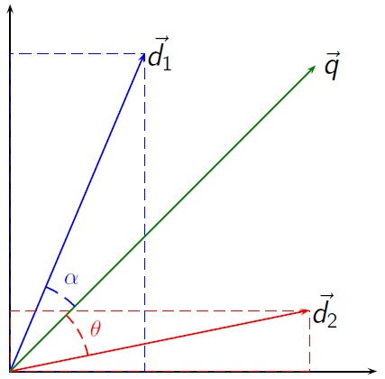
Now we make a simplifying assumption: the occurrence of each word in the document is independent of any other words.  Then if there are t terms, we can plot each document’s vector in a t-dimensional space.  Similarly to the creation of document vectors,  we can convert a keyword query into a t-dimensional query vector by creating a vector with the number of occurrences of each word.  Finally, we can compute a distance between document and query vectors by looking at how closely their vectors match -- by computing the cosine of the angle between the vectors. See the figure to the right (from here) for an example using two dimensions. In this example, q is our query vector and d1 and d2 are the two document vectors. The cosine similarity between one of the document vectors and q would tell us the cosine of the angle between them, which we interpret as how similar the vectors are. The cosine would have value 1 if the vectors exactly match; and it would have value 0 if the vectors were orthogonal.

The cosine similarity between vector dj and q is equal to their dot product divided by the product of their Euclidean norms:

Example. Given the previous document vectors, suppose we are given the query “quick fox.”

The query vector would be: [0, 1, 0, 1, 0, 0, 0, 0, 0, 0, 0] and the cosine similarity for the documents would thus be:

Step 5.1.2. Stopwords and Stemming

The above formulation captures the gist of the techniques.  However, we often decide that some words are of so little value that we should ignore them:  these are stopwords, and we just ignore any word that appears in our stopword list.  (An example above is the word “the.”)  Stopwords need to be ignored in both the query and each document.  Stopwords are typically provided to us by experts in linguistics.

A second issue is that many languages, including English, have many different conjugations and forms of word: e.g., “run -> running -> ran.”  We would like to normalize each word to its core “stem.”  Stemming for English is very complex because of the many different word variations.  We thus need to use specialized algorithms -- like the heuristic Porter’s Stemming Algorithm -- or a more linguistically based technique called lemmatization.  Applying stemming or lemmatization to words in the document and the query will “regularize” them.  In the example above, “doggedly” would be stemmed back to “dog” (which might or might not be helpful in this case!).

All told, an improved version of the technique from Step 5.1.1 parses each word (from the document or query), drops every stop word, and creates a vector of the stemmed / lemmatized words.

Step 5.1.3. Inverse Document Frequency

Still the techniques we’ve described so far have a weakness: they count all (non-stopword) words as being of equal value.  We would like to give rare words more importance than ones found in all documents.  To measure a word’s importance, we will develop a metric called inverse document frequency (idf).  In its simplest form, a word’s idf is a ratio between the total number of documents, and how many documents include a word.  (Note that the idf is independent of a given document -- it is a measure of the word’s popularity across the full set of documents, sometimes called a corpus and represented by the letter D.)  Typically, we don’t directly use the ratio, however -- instead we use its base-10 logarithm.  Thus, we define:

Example. For illustrative simplicity, let’s temporarily ignore stemming and stopwords.  Going back to the example in Step 5.1.1, we can compute an IDF vector for our words and the corpus:

IDF = [0, 0.3, 0.3, 0, 0, 0.3, 0.3, 0.3, 0.3, 0.3, 0.3]

Note that 0.3 is the log of 2 / 1 and 0 is the log of 2/2.

Now, in our above cosine similarity measure, we will use the tf * idf term (not just the tf term) for each word wi, in both the document and query vectors.  The cosine similarity between these vectors will be our measure of relevance or similarity.

Example.  Again without stemming and stopwords, we can match the query “quick fox” and the documents.  Here the word “quick” has 0.3 IDF, and “fox” has 0 IDF (since it appears in both documents).  We will get:

Step 5.2. Initializing Parser Code

Now you’ve seen the basics.  Let’s get started by setting up some tools you’ll find to be helpful in eliminating “grunge” work.  The Natural Language Toolkit (nltk) does a few useful things for you, including parsing sentences with punctuation, as well as stemming.

For this part of the homework, you’ll want to start with the Advanced-Starter Jupyter notebook we’ve given you.  Open it and rename it to Advanced.  Run the first Cell and follow the instructions in the code comments: download the punkt package, which will parse text documents and respect punctuation.  

Now run the remaining Cells until you get to the bottom, where you can write your own code.  At this point, you should have several available data structures useful for writing your code:

1. A dictionary called docs from document name to document content.  Docs has some content pulled from Wikipedia.
2. A set, stopwords, containing (shockingly!) stopwords.
3. A variable MAX_WORDS that is set to the maximum number of words we will consider (after which we’ll ignore all subsequent words).  We can use this to initialize 2D arrays in numpy.
4. A variable stemmer, pointing to an object which you will be able to use to stem words.

Step 5.3. Build Document Vectors

As a first step, you will need to simultaneously build a lexicon (a list of known words, which you will want to map to document vector indices) and a list of document vectors.  You may also want to build an inverse lexicon that maps from position back to word.

Create a 2D array representing the document vectors.  This should have a number of rows equal to the size of the corpus, and a number of columns equal to MAX_WORDS.

Iterate through the various documents in docs.  Call a function doc_vector(content, vector, lexicon, inverse_lexicon, stopwords, word_count) that will calculate the term frequency (tf) for the contents of each document.  Word_count is the number of unique words seen so far. Lexicon and inverse_lexicon are also the current state of the respective dictionaries. Vector should be a blank (read: zeroed) vector that your function will overwrite to contain the document vector for the given content.

Define doc_vector as above.  You can use nltk.word_tokenize() to parse the documents into streams of words.  Make sure you account for variations in capitalization etc.  Remove any “words” that don’t have letters (these are clearly not words! You can call the function has_letter to test this) as well as stop words.  Call stemmer.stem() on a word to get its stem.  For each stem, if necessary extend the lexicon (and inverse lexicon), unless you have already seen MAX_WORDS (if you have seen this, you need to simply ignore the keyword).  Set the term frequency in the appropriate element in the document vector.  Return the updated word_count after you have added any new terms to the lexicon.

Now compute a single vector idf representing, for each word, its idf within the corpus.

Step 5.4. Create Query Vectors

As we described previously, standard search simply takes a keyword query and treats it much as a document.  Write a function create_query_vector(query) that takes a keyword query string, appropriately calls doc_vector to create a query vector, and returns the query vector.

Step 5.5. Produce Ranked Results

Write a function search(vectors, idf, query, num_results) that, when given a 2D array of document vectors, a query vector, and a number num_results:

1. Creates a Pandas DataFrame with schema (docid, docname, score) for the results of matching the query against each document.
2. Uses Numpy multiplication (* between arrays), dot product (@ or np.dotproduct()) and other operations (+, np.linalg.norm() for vector norms, etc) to compute a cosine similarity score for every document.  Add each document ID and score to the DataFrame.
3. Sorts the DataFrame by descending score.
4. Returns the first num_results results.

6.0 Submitting Homework 3

Please sanity-check that your Jupyter notebooks contain both code and corresponding data.  Add the notebook files to hw3.zip using the zip command at the Terminal, much as you did for HW0 and HW1.  The notebooks should be:

• Spark.ipynb
• PageRank.ipynb
• Images.ipynb
• Advanced.ipynb (if applicable)

Next, go to the submission site, and if necessary click on the Google icon and log in using your Google@SEAS or GMail account.  At this point the system should know you are in the appropriate course.  Select CIS 700-003 Homework 3 and upload hw3.zip from your Jupyter folder, typically found under /Users/{myid}.

If you check on the submission site after a few minutes, you should see whether your submission passed validation.  You may resubmit as necessary.